Getting Started

higlass-python is a Python interface for HiGlass. It simplifies authoring HiGlass view configs and offers additional features to load and visualize local datasets as well as extend HiGlass server functionality.

Key features

• Author validated HiGlass view configs with a simplified API

• Render interactive visualizations as standalone HTML or interactive Jupyter Widgets

• Load local, remote, and in-memory datasets via a light-weight, anywidget-based HiGlass server

• Extend HiGlass server with custom tilesets

Example

pip install higlass-python

import higlass as hg

# Remote data source (tileset)
tileset1 = hg.remote(
    uid="CQMd6V_cRw6iCI_-Unl3PQ",
    server="https://higlass.io/api/v1/",
    name="Rao et al. (2014) GM12878 MboI (allreps) 1kb",
)

# Local tileset
tileset2 = hg.cooler("../data/dataset.mcool")

# Create a `hg.HeatmapTrack` for each tileset
track1 = tileset1.track("heatmap")
track2 = tileset2.track("heatmap")

# Create two independent `hg.View`s, one for each heatmap
view1 = hg.view(track1, width=6)
view2 = hg.view(track2, width=6)

# Lock zoom & location for each `View`
view_lock = hg.lock(view1, view2)

# Concatenate views horizontally and apply synchronization lock
(view1 | view2).locks(view_lock)

Whats going on here:

• tileset1 defines a remote tileset (data source), pointing to an exisiting HiGlass server.

• tileset2 defines a local tileset, configuring an anywidget-based HiGlass server to serve tiles from the included cooler file.

• track1 and track2 specify separate hg.HeatmapTrack objects derived from the above tilesets, which are inserted into two separate views (view1 and view2 respectively).

• view_lock is an hg.Lock instance, defining an abstract link between the two views.

• Finally, the two views are concatenated horizontally into a single hg.Viewconf (via the | operator), and lock is used to sync the zoom and location.

Simplest use case

The simplest way to instantiate a HiGlass instance to create a View with an axis Track:

import higlass as hg

hg.view(hg.track("top-axis"))

The hg.track and hg.view utilties provide a flexibile API for creating and composing multiple HiGlass Views and Tracks. The hg.view utility accepts one or more tracks as positional arguments, and view-level properties are specified via keyword-only arguments.

import higlass as hg

hg.view(
    hg.track("top-axis"),
    hg.track("left-axis"),
    width=6,
)

By default, track positions are are inferred via track type but may be overriden or provided explicitly as a tuple of (hg.Track, "top" | "right" | "bottom" | "left").

import higlass as hg

hg.view(
    (hg.track("top-axis"), "top"),
    (hg.track("left-axis"), "left"),
    width=6,
)

Creating a viewconf

At it’s core, higlass-python is a Python interface for authoring and composing validated HiGlass view configs. This core API can be used outside of Jupyter notebooks to load or export HiGlass configurations without any rendering. For example, creating and exporting a view config as JSON:

import higlass as hg

pileup_track = hg.track("pileup").properties(
    data={"type": "bam", "url": "my_bam"},
).opts(
    axisPositionHorizontal="right",
)
view = hg.view(hg.track("top-axis"), (pileup_track, "top"))
view.viewconf().json() # or .dict() for a Python dict

# {
#   "editable": true,
#   "viewEditable": true,
#   "tracksEditable": true,
#   "views": [
#     {
#       "layout": { "x": 0, "y": 0, "w": 12, "h": 6 },
#       "tracks": {
#         "top": [
#           {
#             "type": "top-axis",
#             "uid": "5f8433fc-9b7a-48a2-b4c3-bccddf8a0bee"
#           },
#           {
#             "type": "pileup",
#             "uid": "68405ebc-08b2-469a-ab96-ea7925a39ae2",
#             "options": {
#               "axisPositionHorizontal": "right"
#             },
#             "data": {
#               "type": "bam",
#               "url": "my_bam"
#             }
#           }
#         ]
#       },
#       "uid": "2d774b94-fc5d-49c2-9c51-bbad9fa6e73f",
#       "zoomLimits": [1, null]
#     }
#   ]
# }

or loading an existing view config via URL to access a sub-track:

import higlass as hg

viewconf = hg.Viewconf.from_url("https://higlass.io/api/v1?d=default")
viewconf.views[0].tracks.top[0].json()

# {
#   "tilesetUid": "OHJakQICQD6gTD7skx4EWA",
#   "server": "//higlass.io/api/v1",
#   "type": "horizontal-gene-annotations",
#   "uid": "OHJakQICQD6gTD7skx4EWA",
#   "height": 60,
#   "options": {
#     "name": "Gene Annotations (hg19)"
#   }
# }

Add Genome Position SearchBox

import higlass as hg

mm10 = hg.remote(
    uid="QDutvmyiSrec5nX4pA5WGQ",
    server="//higlass.io/api/v1",
)

view1 = hg.view(

    mm10.track("gene-annotations",height=150).opts(
        minHeight = 24,
    ),
    genomePositionSearchBox = hg.GenomePositionSearchBox(
        autocompleteServer="//higlass.io/api/v1",
        autocompleteId="OHJakQICQD6gTD7skx4EWA",
        chromInfoId="hg19",
        chromInfoServer="//higlass.io/api/v1",
        visible=True)
)

#In order to get access to track sources from higlass.io data sources
list_of_track_source_servers = [
    "//higlass.io/api/v1",
    "https://resgen.io/api/v1/gt/paper-data"
  ]

view1.viewconf(trackSourceServers = list_of_track_source_servers, exportViewUrl = "/api/v1/viewconfs")

View extent

The extent of a view can be set using the hg.View.domain() method, either in 1D:

import higlass as hg

view = hg.view(hg.track("top-axis")).domain(x=[0, 1e7])

or 2D:

import higlass as hg

view = hg.view(hg.track("heatmap")).domain(x=[0, 1e7], y=[0, 1e7])

Track Types

A list of available track types can be found in the documentation for HiGlass. Based on the tileset data type, we can sometimes provide a recommended track type as well as a recommended position.

import higlass as hg

tileset = hg.cooler("./data.mcool")
track = tileset.track() # defaults to 'heatmap'
view = hg.view(track)   # defaults to 'center' position

Combining Tracks

Overlaying tracks

Tracks may be combined with the hg.combine() utility:

import higlass as hg

tileset = hg.remote(
    uid="F2vbUeqhS86XkxuO1j2rPA",
    server="//higlass.io/api/v1",
)

combined_track = hg.combine(
    hg.track("top-axis"),
    tileset.track("horizontal-bar")
)

hg.view((combined_track, "top")).domain(x=[0, 1e9])

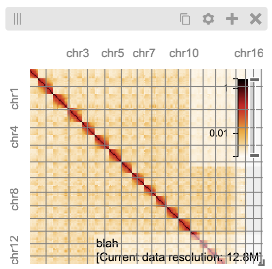
Chromosome grid on a heatmap

import higlass as hg

cs_ts = hg.chromsizes('chromSizes_hg19_reordered.tsv')
cool_ts = hg.cooler("Dixon2012-J1-NcoI-R1-filtered.100kb.multires.cool")

hg.view(
    (hg.combine(
        cool_ts.track(options={"name": "blah"}),
        cs_ts.track('2d-chromosome-grid'),
    position='center'), 'center'),
    (cs_ts.track('horizontal-chromosome-labels'), 'top'),
    (cs_ts.track('horizontal-chromosome-labels'), 'left'),
    width=6)

Multiple Views

Multiple views are instantiated separately and can be arranged on a grid that is 12 units wide and an arbitrary number of units high. To create two side by side views, set both to be 6 units wide and use the | operator to concatenate horizontally. The / operator can be used to stack vertically.

import higlass as hg

view1 = hg.view(hg.track("top-axis"), width=6)
view2 = hg.view(hg.track("top-axis"), width=6)

view1 | view2

Synchronization

Views and track can be synchronized by location, zoom level and values scales.

Zoom and Location locks

Location locks ensure that when one view is panned, all synchronized views pan with it. Zoom locks do the same with zoom level. Locks are specified by linking two or more views together via the hg.lock utility, and then passing the created lock to hg.Viewconf.locks().

lock = hg.lock(view1, view2)
(view1 | view2).locks(lock)

Both zoom and location are synchronized by default, but locks can be applied specifically via the zoom or location keyword arguments:

lock = hg.lock(view1, view2)

(view1 | view2).locks(lock) # both zoom and location

(view1 | view2).locks(zoom=lock) # zoom only

(view1 | view2).locks(location=lock) # location only

Viewport Projection

Viewport projections can be applied via the hg.View.project() method. This method creates a new track with the viewport bounds of one view and appends this newly created track onto another view (i.e., a projection).

view1 = hg.view(track1, width=6)
view2 = hg.view(track2, width=6)

view1.project(view2, to="center") | view2

Note that viewport projections always need to be paired with other non- viewport projections. Multiple ViewportProjection tracks can, however, be combined, as long as they are associated with regular tracks.

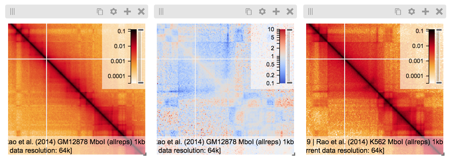
Dataset Arithmetic

HiGlass supports client-side division between quantitative datasets with a “divided” track. This makes it possible to quickly compare two datasets by visualizing their ratio as computed on loaded tiles rather than the entire dataset:

hg.divide(
    tileset1.track("heatmap"),
    tileset2.track("heatmap"),
)

A full example can be found below:

tset1 = hg.remote(
    uid="CQMd6V_cRw6iCI_-Unl3PQ",
    name="Rao et al. (2014) GM12878 MboI (allreps) 1kb",
)

tset2 = hg.remote(
    uid="QvdMEvccQuOxKTEjrVL3wA",
    name="Rao et al. (2014) K562 MboI (allreps) 1kb",
)

t1 = tset1.track("heatmap", height=300)
t2 = tset2.track("heatmap", height=300)

t3 = hg.divide(t1, t2).opts(
    colorRange=["blue", "white", "red"],
    valueScaleMin=0.1,
    valueScaleMax=10,
)

domain = (7e7, 8e7)
v1 = hg.view(t1, width=4).domain(x=domain)
v2 = hg.view(t2, width=4).domain(x=domain)
v3 = hg.view(t3, width=4).domain(x=domain)

(v1 | v3 | v2).locks(hg.lock(v1, v2, v3))

Other Examples

The examples below demonstrate how to use the HiGlass Python API to view data locally in a Jupyter notebook or a browser-based HiGlass instance.

Jupyter HiGlass Component

To instantiate a HiGlass component within a Jupyter notebook, we first need to specify which data should be loaded. This is accomplished either by specifying a local tileset (via hg.cooler, hg.bigwig, hg.multivec, hg.hitile, hg.bed2ddb) or connecting to an existing HiGlass Server with hg.remote():

import higlass as hg

tileset = hg.remote(
    uid="CQMd6V_cRw6iCI_-Unl3PQ",
    server="http://higlass.io/api/v1/",
)

view = hg.view(
    hg.track("top-axis"),
    tileset.track("heatmap", height=250).opts(
        valueScaleMax=0.5,
    ),
)

Remote bigWig Files

bigWig files can be loaded either from the local disk or from remote http servers. The example below demonstrates how to load a remote bigWig file from the UCSC genome browser’s archives. Note that this is a network-heavy operation that may take a long time to complete with a slow internet connection.

import higlass as hg

tileset = hg.bigwig(
    'http://hgdownload.cse.ucsc.edu/goldenpath/hg19/encodeDCC/'
    'wgEncodeSydhTfbs/wgEncodeSydhTfbsGm12878InputStdSig.bigWig')

hg.view(tileset.track("horizontal-bar"))

For a better user experience, we recommend downloading the data locally first.

!wget http://hgdownload.cse.ucsc.edu/goldenpath/hg19/encodeDCC/wgEncodeSydhTfbs/wgEncodeSydhTfbsGm12878InputStdSig.bigWig

import higlass as hg

tileset = hg.bigwig('./wgEncodeSydhTfbsGm12878InputStdSig.bigWig')

hg.view(tileset.track("horizontal-bar"))

Serving local data

To enable the viewing of local data, higlass-python runs a temporary light-weight HiGlass server in a background thread. This temporary server is only started if a local tileset is used and will only persist for the duration of the Python session.

Cooler Files

We provide a top-level convenience function, hg.cooler, for adding cooler tilesets to the background server:

import higlass as hg

# Adds a tileset to a background HiGlass server
tileset = hg.cooler("../data/Dixon2012-J1-NcoI-R1-filtered.100kb.multires.cool")

# View the local tileset
hg.view(tileset.track("heatmap"))

The background server is exposed globally and may be configured with other custom tilesets.

import higlass as hg

# add a custom tileset manually
ts_custom = hg.server.add(MyCustomTileset())

# calls hg.server.add() internally
ts = hg.cooler("../data/Dixon2012-J1-NcoI-R1-filtered.100kb.multires.cool")

v1 = hg.view(ts.track("heatmap"), width=6)
v2 = hg.view(ts_custom.track("heatmap"), width=6)

v1 | v2

You can clear all active server resources by reseting the server:

hg.server.reset()

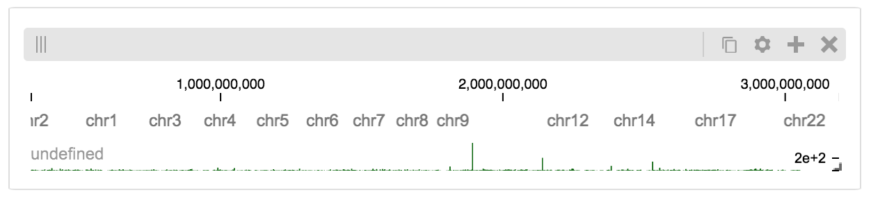
BigWig Files

The top-level hg.bigwig utility is available for viewing local bigWig files. The returned tileset can be used to create both a chromosome labels track and a horizontal bar track for these data.

import higlass as hg

ts = hg.bigwig("../data/wgEncodeCaltechRnaSeqHuvecR1x75dTh1014IlnaPlusSignalRep2.bigWig")

hg.view(
    hg.track("top-axis"),
    ts.track("chromosome-labels"),
    ts.track("horizontal-bar"),
)

Serving custom data

To display data, we need to define a tileset. Tilesets define two functions: info:

> from higlass.tilesets import bigwig
> ts1 = bigwig('http://hgdownload.cse.ucsc.edu/goldenpath/hg19/encodeDCC/wgEncodeSydhTfbs/wgEncodeSydhTfbsGm12878InputStdSig.bigWig')
> ts1.info()
{
 'min_pos': [0],
 'max_pos': [4294967296],
 'max_width': 4294967296,
 'tile_size': 1024,
 'max_zoom': 22,
 'chromsizes': [['chr1', 249250621],
                ['chr2', 243199373],
                ...],
 'aggregation_modes': {'mean': {'name': 'Mean', 'value': 'mean'},
                       'min': {'name': 'Min', 'value': 'min'},
                       'max': {'name': 'Max', 'value': 'max'},
                       'std': {'name': 'Standard Deviation', 'value': 'std'}},
 'range_modes': {'minMax': {'name': 'Min-Max', 'value': 'minMax'},
                 'whisker': {'name': 'Whisker', 'value': 'whisker'}}
 }

and tiles:

> ts1.tiles(['x.0.0'])
[('x.0.0',
  {'min_value': 0.0,
   'max_value': 9.119079544037932,
   'dense': 'Rh25PwcCcz...',   # base64 string encoding the array of data
   'size': 1,
   'dtype': 'float32'})]

The tiles function will always take an array of tile ids of the form id.z.x[.y][.transform] where z is the zoom level, x is the tile’s x position, y is the tile’s y position (for 2D tilesets) and transform is some transform to be applied to the data (e.g. normalization types like ice).

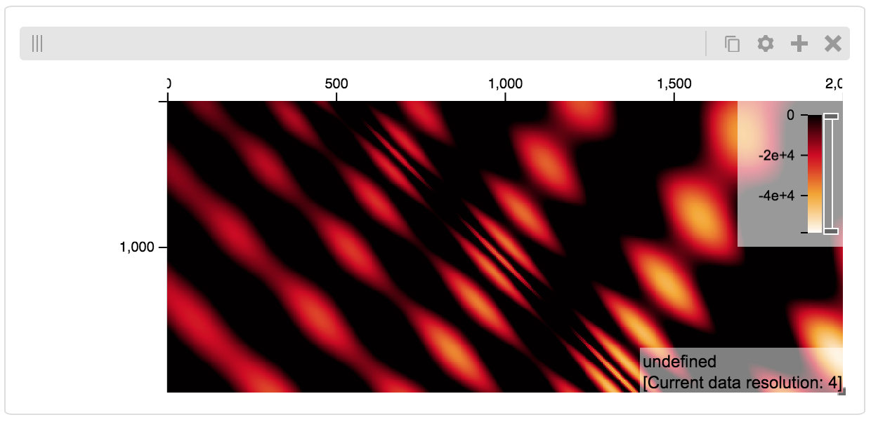
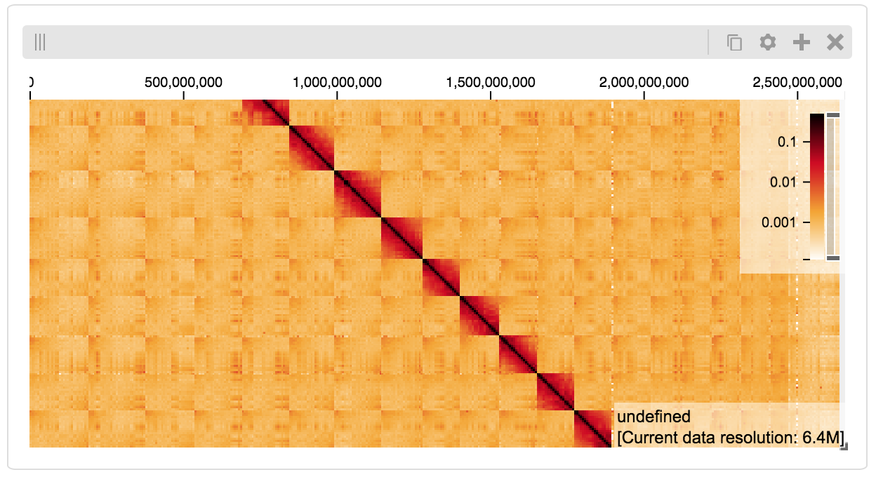
Numpy Matrix

By way of example, let’s explore a numpy matrix by implementing the info and tiles functions described above. To start let’s make the matrix using the Eggholder function.

import numpy as np

dim = 2000
I, J = np.indices((dim, dim))
data = (
    -(J + 47) * np.sin(np.sqrt(np.abs(I / 2 + (J + 47))))
    - I * np.sin(np.sqrt(np.abs(I - (J + 47))))
)

Then we can define the data and tell the server how to render it.

import higlass as hg
from  clodius.tiles import npmatrix
from higlass.tilesets import LocalTileset

ts = hg.server.add(
    LocalTileset(
        info=lambda: npmatrix.tileset_info(data),
        tiles=lambda tids: npmatrix.tiles_wrapper(data, tids),
        uid="example-npmatrix",
        datatype="matrix",
    )
)

hg.view(
    hg.track("top-axis"),
    hg.track("left-axis"),
    ts.track("heatmap", height=250).opts(valueScaleMax=0.5),
)